head(max_stats)

##                          Name HP ATK SPD DEF RES BST WeaponType MoveType
## 1                        Abel 39  33  32  25  25 154 Blue Lance  Cavalry
## 2                     Alfonse 43  35  25  32  22 157  Red Sword Infantry
## 3 Alfonse (Hares at the Fair) 41  35  33  30  18 157  Green Axe  Cavalry
## 4                         Alm 45  33  30  28  22 158  Red Sword Infantry
## 5                      Amelia 47  34  34  35  23 173  Green Axe  Armored
## 6                        Anna 41  29  38  22  28 158  Green Axe Infantry

Distributions

Let’s start by looking at the distributions of each stat type to see how these values are spread out. I’ll remove the BST (base stat total) column for now. If you remember from my previous post, the BST is the sum of all other stats, and therefore it has a different range of values, which will get in the way of our visualization.

melt_stats <- melt(max_stats[, -7]) # Removing the BST column
ggplot(data=melt_stats, aes(value)) +
    geom_density(size=1, color="red") +
    facet_grid(~variable) +
    theme_few() +
    xlab("Value") +
    ylab("Density") +
    ggtitle("Stat densities") +
    theme(plot.title = element_text(hjust = 0.5))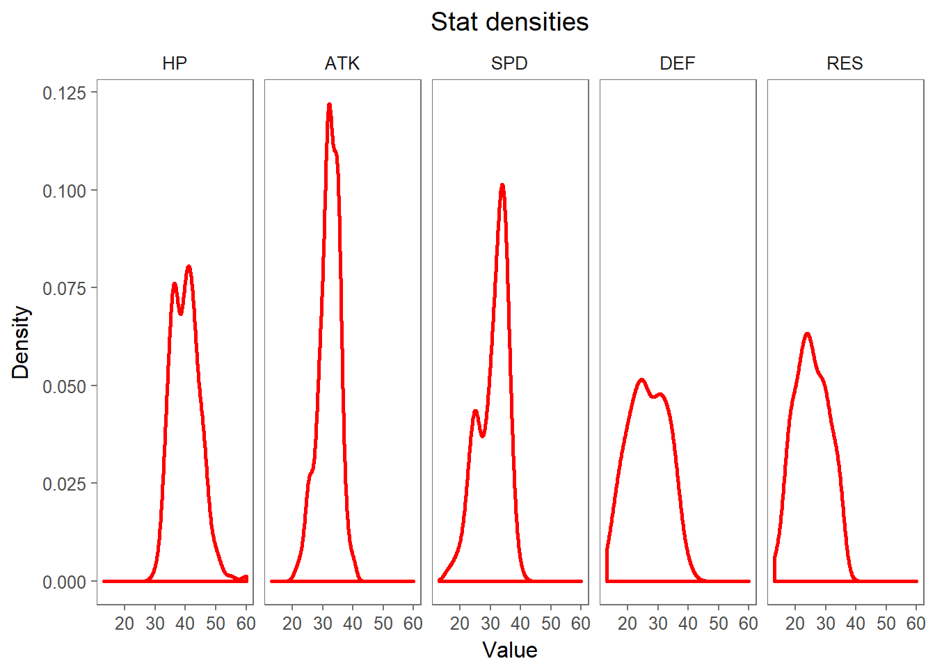

We can see that most heroes have an ATK stat of around 32, and that this stat’s distribution is not very wide, meaning that there is not that big a difference between individual units’ offensive power. The DEF stat, however, seems to be a bit more distributed among the characters. We can, of course, compute each stat’s variance and observe this.

var(max_stats$ATK)

## [1] 11.82872

var(max_stats$DEF)

## [1] 40.5983

Anyway, let’s take a quick look at the BST column now. This can give us a quick-and-dirty idea of a unit’s overall power. It’s worth noting that the BST is also used by the game as a classification measure when pairing up players against each other in the Arena mode of the game, where players using characters with higher BSTs are pitted against each other. It also reflects in the number of points you get in the Arena, which allows you to challenge even stronger players given time. So let’s take a look at the heroes with the highest BST scores, which will maximize our Arena score (without considering other BST increasing factors, such as weapon power and skills).

top_heroes <- max_stats[order(max_stats$BST, decreasing = F), ]
top_heroes <- tail(top_heroes, 20)

ggplot(top_heroes, 
       aes(factor(top_heroes$Name, levels=top_heroes$Name), BST)) +
    geom_bar(stat="identity", fill="red") +
    coord_flip() + 
    scale_y_continuous(limits=c(0, 190), breaks=seq(0, 190, 20)) +
    ggthemes::theme_few() +
    xlab("Heroes") +
    ggtitle("Top 20 heroes with highest BST") +
    theme(plot.title = element_text(hjust = 0.5))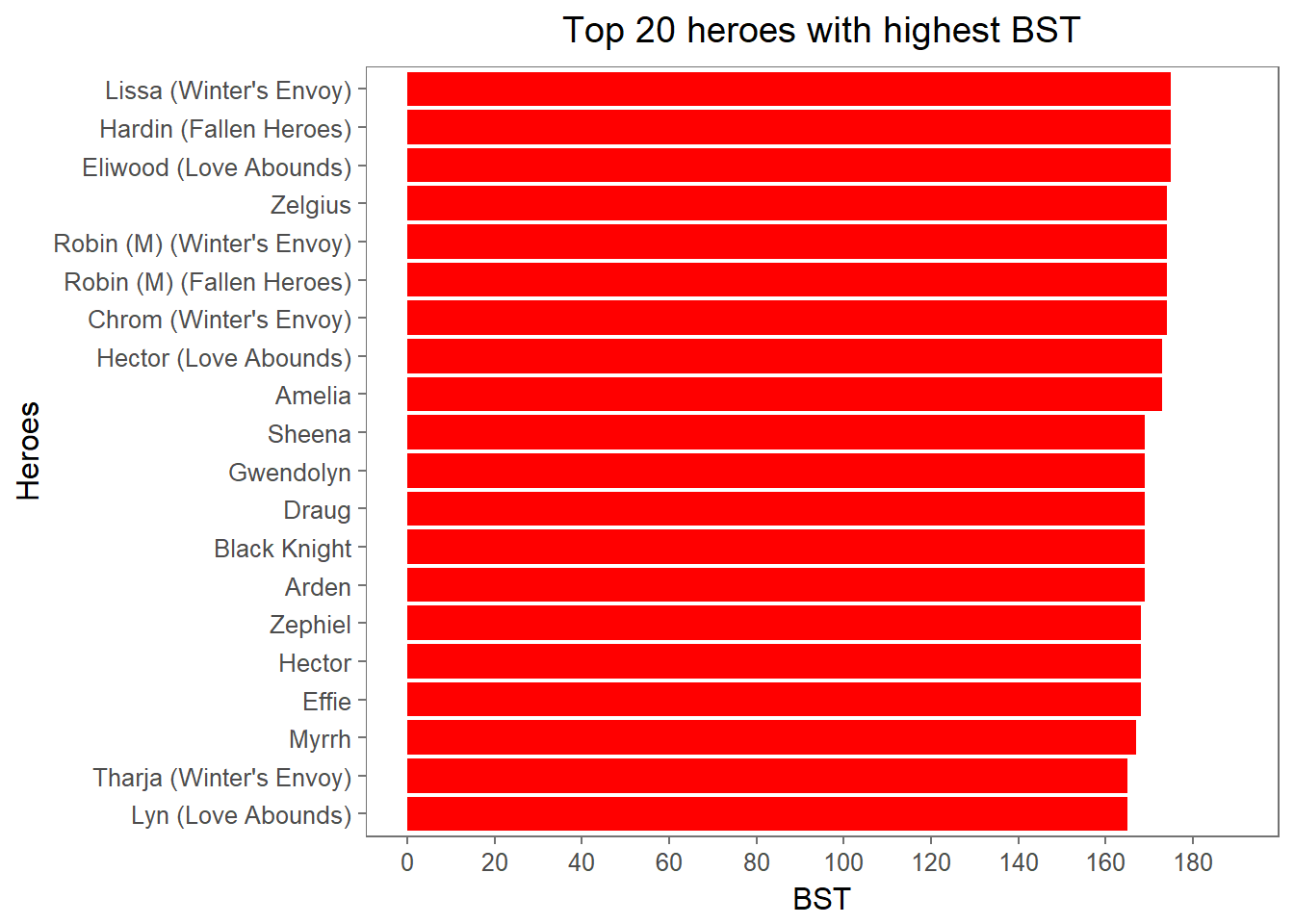

The barplot we just created might not seem very informative at first, given the similar BST values shown, but we do find something interesting once we include units’ movement type information:

ggplot(top_heroes, 
       aes(factor(top_heroes$Name, levels=top_heroes$Name), BST, fill=MoveType)) +
    geom_bar(stat="identity") +
    coord_flip() + 
    scale_y_continuous(limits=c(0, 190), breaks=seq(0, 190, 20)) +
    ggthemes::theme_few() +
    xlab("Heroes") +
    ggtitle("Top 20 heroes with highest BST + move type") +
    theme(plot.title = element_text(hjust = 0.5))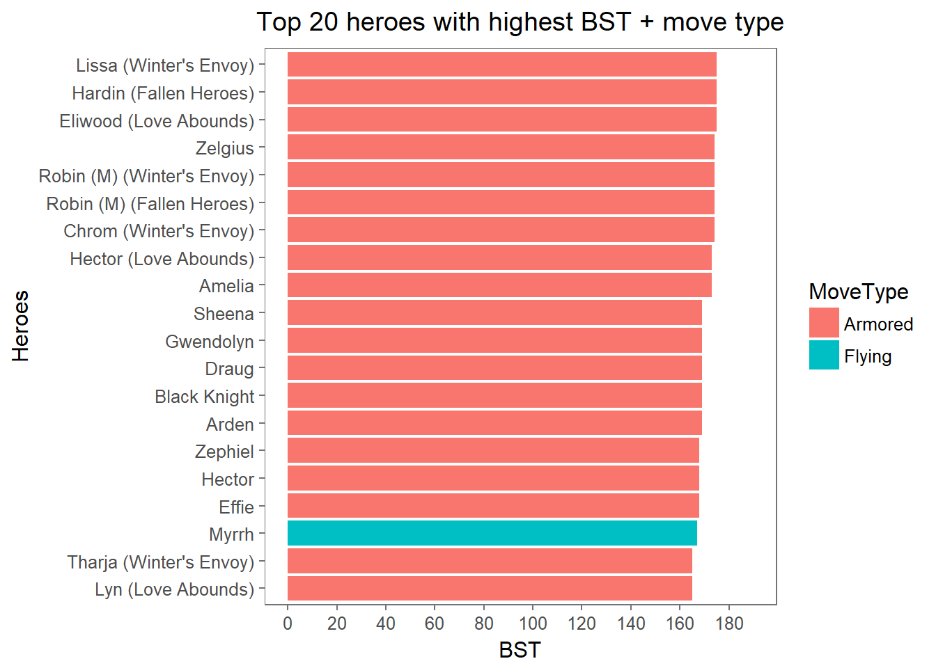

Armored units have the highest BST! …This really should not come as a surprise to most players; the whole idea of the Armored class is to have higher stats than average to compensate for their limited movement. One cool thing of note though is the inclusion of Myrrh, a flying type unit, in our top 20 BST list. Myrrh is a “Breath” weapon user (a.k.a. a dragon manakete), which explains a bit why her BST is higher than average (although the next highest “Breath” user, Nowi, only appears at #30, 12 units below).

Clustering analysis

Let’s try using some clustering analysis techniques to see if we can find any kind of cluster of units based on their stats. With this we should be able to identify similarly built characters or archetypes. First we’ll calculate the correlations between each hero’s stats to see how close each of them are. Then, we can use agglomerative clustering with the hclust function and euclidean distance to group our characters and visualize them in a dendrogram. Let’s remove our categorical variables and the BST column for now.

stats_only <- max_stats[, -c(7, 8, 9)]
rownames(stats_only) <- stats_only$Name
stats_only$Name <- NULL

stats_cor <- cor(t(stats_only))

d <- proxy::dist(stats_cor, method="euclidean")
fit <- hclust(d, method="ward.D")
dend <- ggdendro::dendro_data(fit)

dend_order <- fit$labels[fit$order]

dendro <-
    ggdendro::ggdendrogram(dend, rotate=FALSE) +
    scale_x_continuous(expand = c(0, 0.5), 
                       labels=dend_order, 
                       breaks=1:length(dend_order)) +
    scale_y_continuous(expand = c(0.02, 0)) +
    ggtitle("Hero similarity dendrogram") +
    theme(plot.title = element_text(hjust = 0.5))

dendro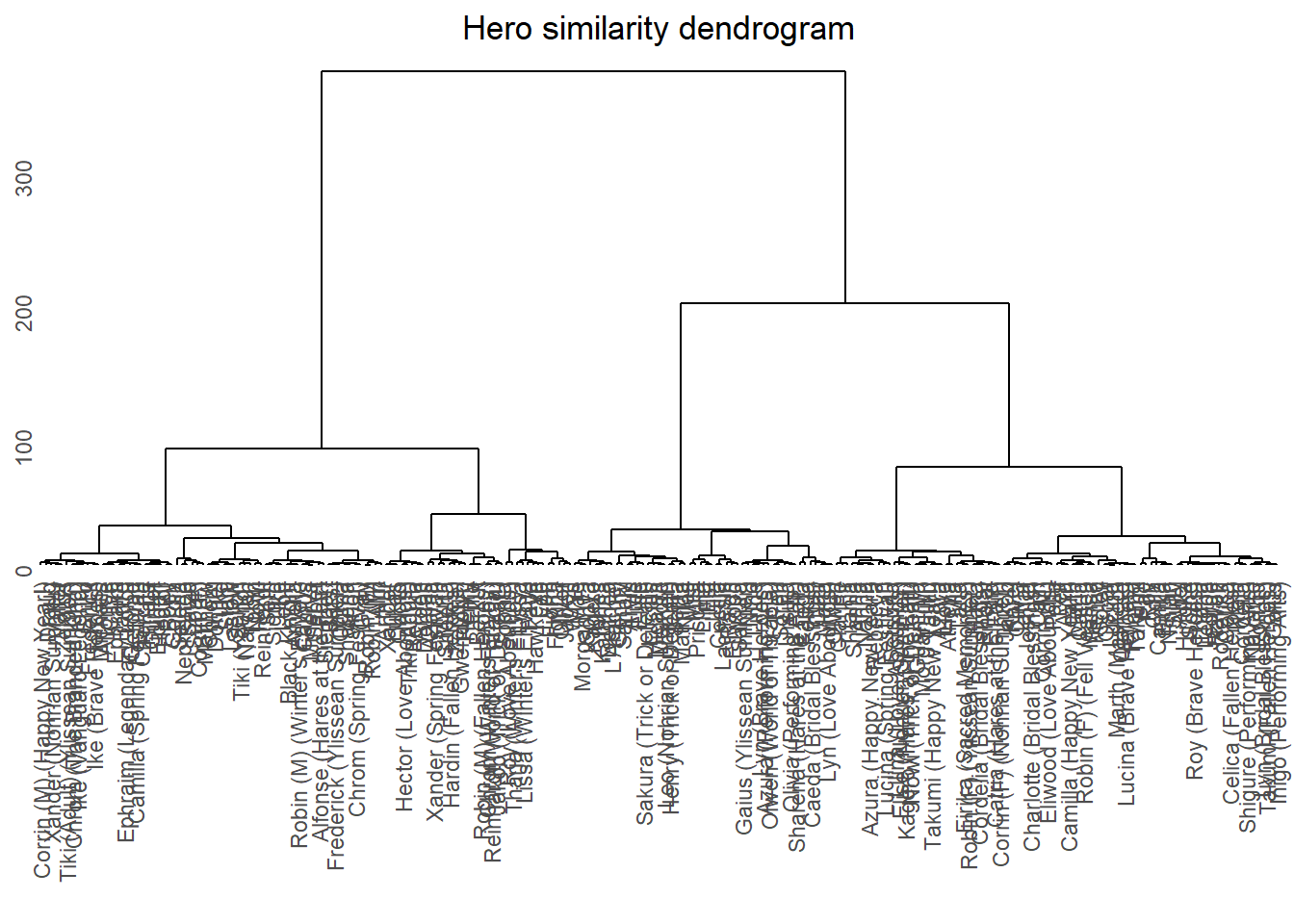

I’ll use the cutreeDynamic function from the dynamicTreeCut package to cut our dendrogram into clusters. This package attempts to automatically define the best number of clusters based on the shape of the dendrogram, so we don’t have to worry about selecting an aribitrary number of clusters. I’ll also use the labels2colors function from the WGCNA package to obtain a color for each cluster underneath the dendrogram. These packages were originally developed to visualize clusters of genes in Bioinformatics analyses. Gotta love that interdisciplinarity!

The WGCNA package also provides a function with base R to plot the dendrogram with colors, but since I prefer ggplot2, I’ll be using a few functions from the grid and gridExtra packages. A BIG shout out to the StackOverflow members in this and this topic for the insights in how to align a dendrogram and how to combine and align two ggplot graph images.

dynamicMods <- dynamicTreeCut::cutreeDynamic(dendro=fit)                   
dynamicColors <- WGCNA::labels2colors(dynamicMods)

out <- data.frame(chars=rownames(stats_only), 
                  modules=dynamicMods, 
                  colors=dynamicColors,
                  stringsAsFactors=FALSE)

out <- out[match(dend_order, out$chars), ]

clusters <- ggplot(out, aes(factor(chars, levels=chars), y=1, fill=colors)) +
            geom_tile() +
            scale_fill_identity() +
            scale_y_continuous(expand=c(0, 0)) +
            theme(axis.title=element_blank(),
                axis.ticks=element_blank(),
                axis.text=element_blank(),
                legend.position="none",
                plot.title = element_text(hjust = 0.5))

gp1 <- ggplot2::ggplotGrob(dendro)
gp2 <- ggplot2::ggplotGrob(clusters)

maxWidth <- grid::unit.pmax(gp1$widths[2:5], gp2$widths[2:5])
gp1$widths[2:5] <- as.list(maxWidth)
gp2$widths[2:5] <- as.list(maxWidth)
g <- gridExtra::arrangeGrob(gp1, gp2, ncol=1,heights=c(9/10, 1/10))
grid::grid.draw(g)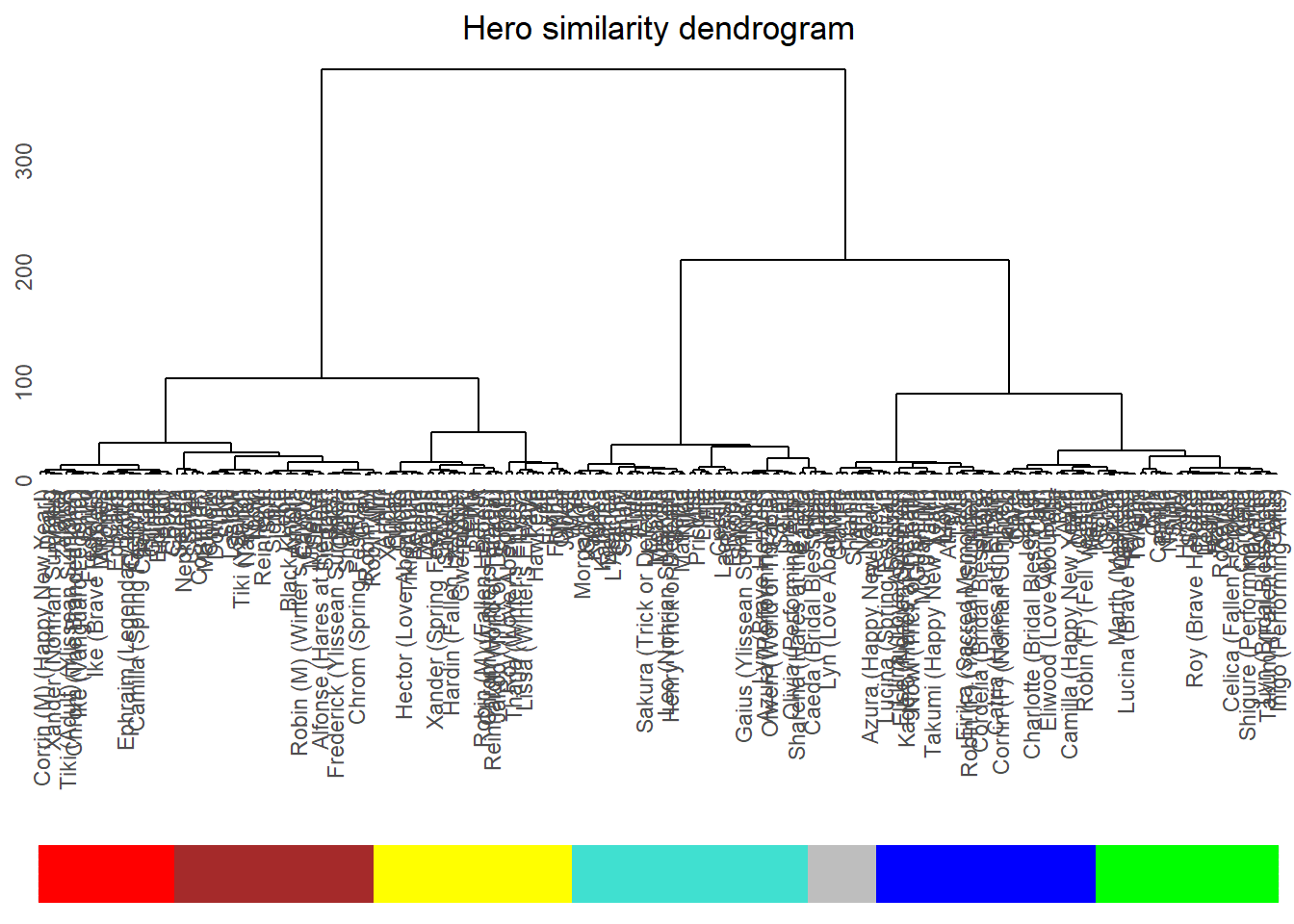

As we can see we got 7 nice clusters, with the turquoise cluster being the largest. As a side note, the dynamicTreeCut package reserves the “grey” color for elements which weren’t able to be assigned to any other cluster. Usually, one would discard this group, but I’ll keep it in this analysis just so we don’t lose any hero. Let’s include cluster information into our data and take a look at a few boxplots so we can get a feel for each cluster.

max_stats$label <- dynamicColors

max_stats2 <- max_stats
max_stats2$BST <- NULL

melt_stats2 <- melt(max_stats2)

ggplot(melt_stats2, aes(value)) +
    geom_boxplot(aes(x=variable, y=value, fill=variable)) +
    facet_grid(~label) + 
    theme_few() +
    theme(legend.title=element_blank(),
          legend.position = "bottom",
          axis.title=element_blank(), 
          axis.text.x=element_blank(),
          axis.ticks.x=element_blank(),
          plot.title = element_text(hjust = 0.5)) +
    ggtitle("Stat boxplots by cluster")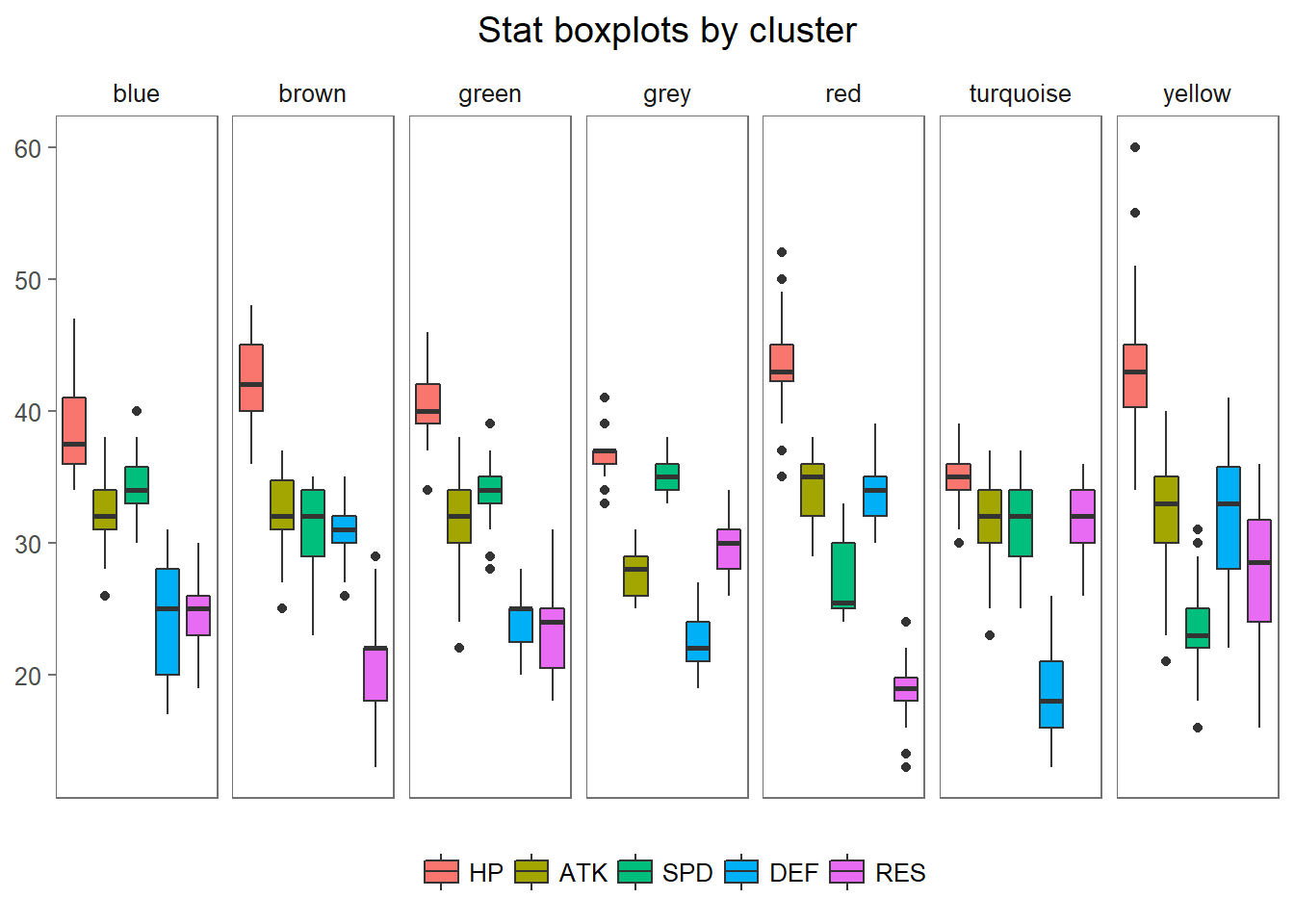

We can also do principal component analysis to see how our clusters represent (most of) the variability of the data. We can see it’s not perfect, but there does seem to be some sense in our clustered points.

pca <- prcomp(stats_only)

df_out <- as.data.frame(pca$x)
df_out$label <- max_stats$label
head(df_out)

##                                   PC1       PC2       PC3        PC4
## Abel                        -1.727858  1.253100 -1.148936 -0.6118986
## Alfonse                      8.626724 -2.674268 -2.592615 -0.7335428
## Alfonse (Hares at the Fair)  5.765115  6.114256 -2.334997 -1.8918197
## Alm                          5.058571  1.167998 -1.279048  2.4418803
## Amelia                       9.378496  2.547198  2.816638 -1.8185376
## Anna                        -6.465976  3.767082  3.455966  2.1557244
##                                     PC5  label
## Abel                        -0.33728966  green
## Alfonse                      1.16584188    red
## Alfonse (Hares at the Fair)  0.08645923  brown
## Alm                         -1.94807904 yellow
## Amelia                      -5.88638553  brown
## Anna                        -4.38269169   grey

ggplot(df_out,aes(x=PC1, y=PC2, color=label)) +
    scale_color_identity() +
    geom_point(size = 5) + 
    theme_few() +
    ggtitle("Principal Component Analysis") +
    theme(plot.title = element_text(hjust = 0.5))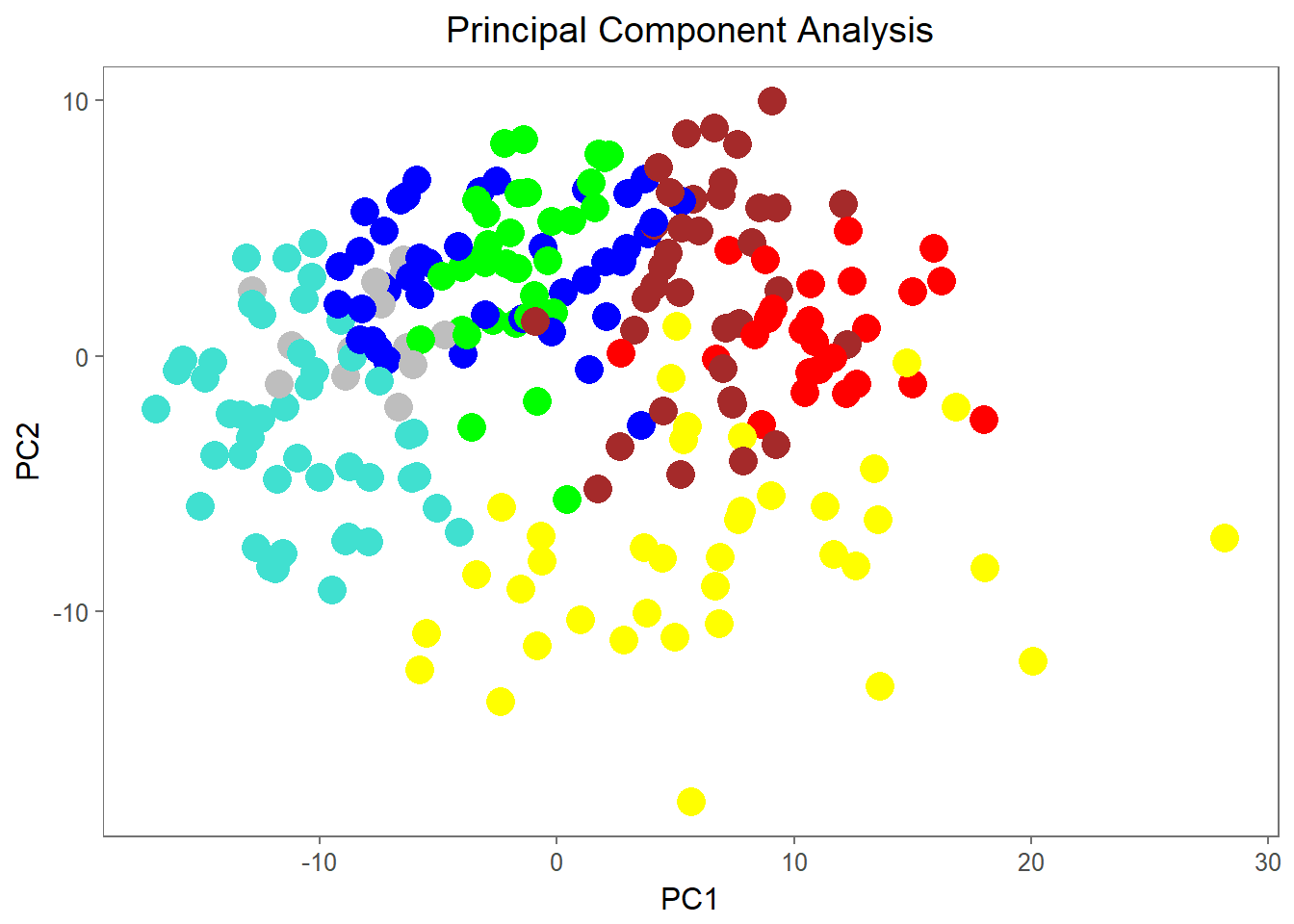

We can use geom_text to check out the units in each cluster:

ggplot(df_out,aes(x=PC1, y=PC2, color=label)) +
    scale_color_identity() +
    geom_point(size = 5) + 
    geom_text(label=rownames(df_out), size=3, color="black") +
    theme_few() +
    ggtitle("Principal Component Analysis") +
    theme(plot.title = element_text(hjust = 0.5))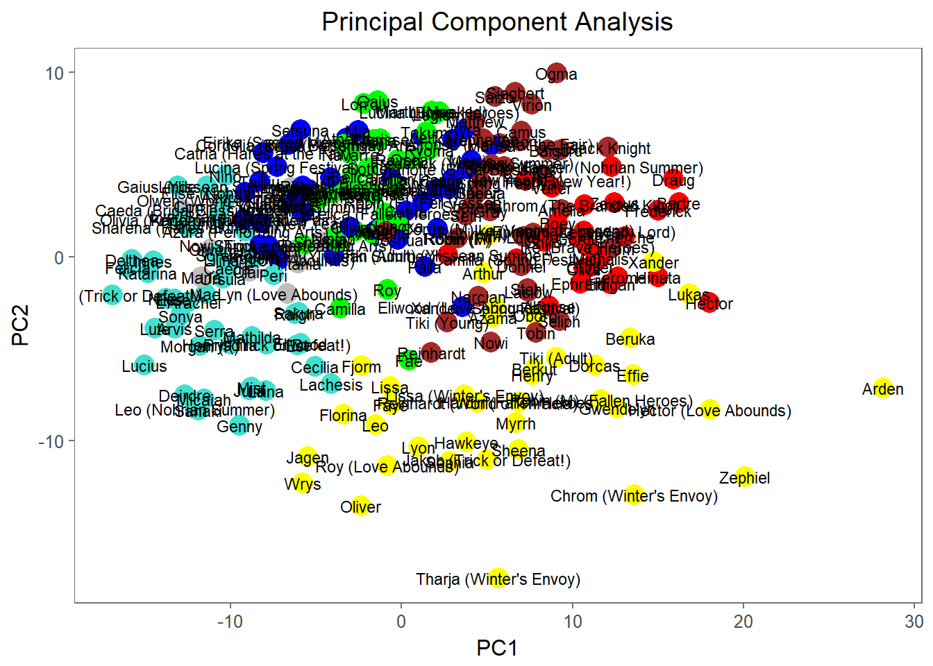

We can now use the by function to find the average stats of heroes within each cluster:

stats_label <- as.data.frame(cbind(stats_only, max_stats$label))
names(stats_label) <- c("HP", "ATK", "SPD", "DEF", "RES", "label")
res <- by(stats_label[, 1:5], stats_label$label, colMeans)

The stats inside each element of the res list are the average stats of the heroes within each cluster. We can consider these stats, therefore as a sort of representative character for each color group. Let’s try to see now which hero within each cluster is the closest to this average. To do this, we’ll take each group of heroes, subtract the stats of our average hero and take the absolute value of the results, average them for each hero to get a distance measure, and see which hero has the lowest distance.

reps <- sapply(unique(as.character(stats_label$label)), USE.NAMES=FALSE, function(color){
    color_rep <- res[[color]]
    color_chars <- stats_label[stats_label$label == color,]
    color_chars$label <- NULL
    diff_df <- t(abs(t(color_chars) - color_rep))
    char_dist <- rowSums(diff_df)/ncol(diff_df)
    closest_char <- char_dist[which.min(char_dist)]
})

reps_df <- as.data.frame(cbind(unique(as.character(stats_label$label)), reps))
names(reps_df) <- c("cluster", "distance_to_mean")
reps_df

##                                cluster  distance_to_mean
## Roderick                         green 0.514285714285715
## Michalis                           red 0.630769230769231
## Sharena                          brown  1.05789473684211
## Reinhardt (World of Thracia)    yellow  1.68421052631579
## Titania                           grey 0.861538461538463
## L'Arachel                    turquoise  1.10222222222222
## Catria                            blue  1.33809523809524

We can now take a look at our PCA plot again and check that our representative heroes lie somewhat centralized in their own clusters:

reps <- rownames(reps_df)
chars <- rownames(df_out)

chars[!chars %in% reps] <- ""

ggplot(df_out,aes(x=PC1, y=PC2, color=label)) +
    scale_color_identity() +
    geom_point(size = 5) + 
    geom_text_repel(label=chars, size=3, color="black") +
    theme_few() +
    ggtitle("Principal Component Analysis") +
    theme(plot.title = element_text(hjust = 0.5))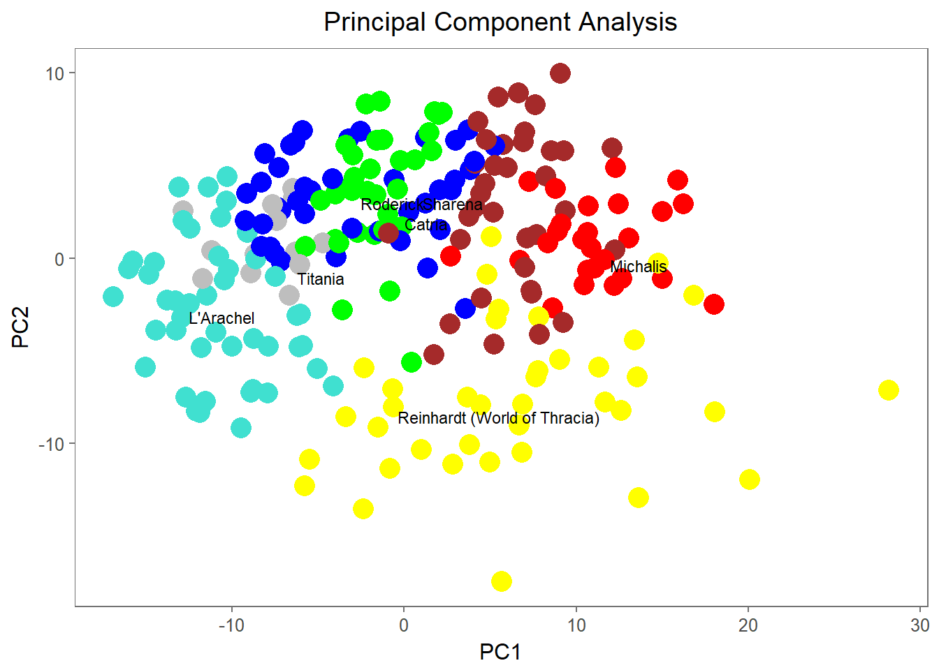

To finish things off, let’s take a look at how movement and weapon types are arranged within each cluster. I couldn’t really decide on a better way to visualize this information, so here are two I could come up with:

A faceted stacked barplot

ggplot(max_stats, aes(x=factor(WeaponType))) +
    geom_bar(stat="count", aes(fill=max_stats$MoveType)) +
    xlab(label="Weapon type") +
    ylab(label="Count") +
    theme(legend.title = element_blank(),
          plot.title = element_text(hjust = 0.5)) + 
    coord_flip() +
    facet_wrap(~label) +
    ggtitle("Movement and weapon types by cluster")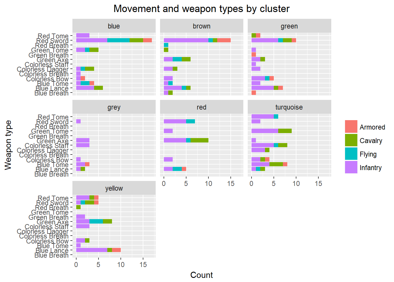

A faceted bubble chart (once again, thanks to SO for this link)

counts <- paste(max_stats$WeaponType, max_stats$MoveType, max_stats$label)

max_stats$category <- counts
max_stats$size <- as.numeric(table(max_stats$category)[max_stats$category])
max_stats$radius <- sqrt(max_stats$size / pi)

ggplot(max_stats, aes(x=factor(WeaponType), y=MoveType)) +
    geom_point(aes(size=radius*7.5), shape=21, fill="white") + 
    geom_text(aes(label=size), size=4, color = "black") +
    scale_size_identity() +
    xlab(label="Weapon type") +
    ylab(label="Move type") +
    theme(axis.text.x = element_text(angle=90),
          plot.title = element_text(hjust = 0.5)) + 
    facet_wrap(~label) +
    ggtitle("Movement and weapon types by cluster")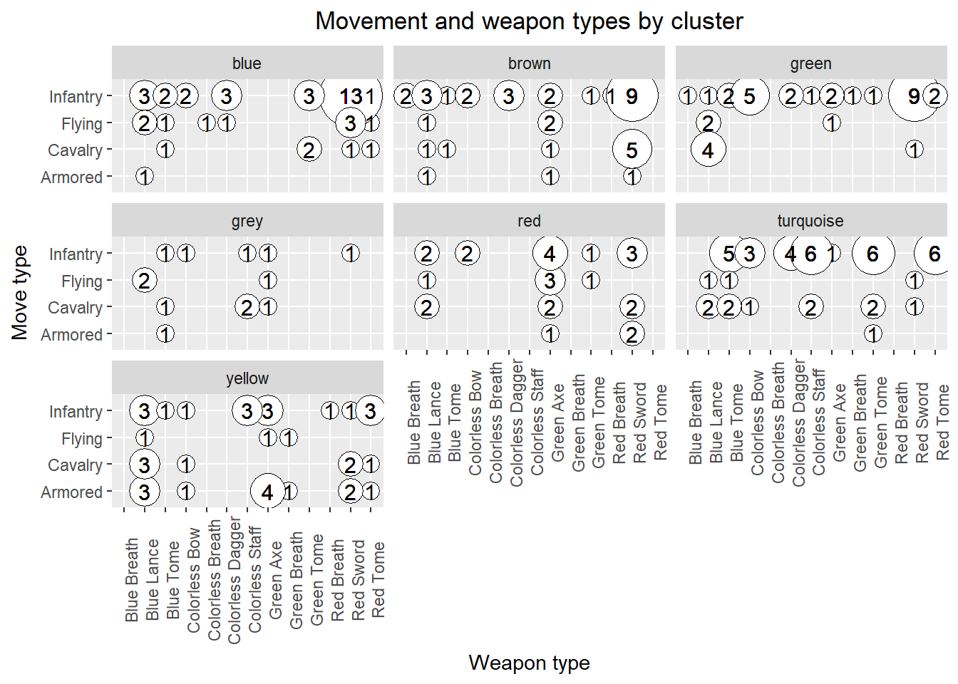

These plots give us a pretty good idea about the composition of each of our clusters. We can see that while Red Sword Infantry characters are dominant in the cast, they’re mostly concentrated in the blue, brown and green clusters. Also, the yellow group seems to be where most armored users wound up. Finally, the most common characters in the turquoise group are mages and staff users. As we can see in our previous boxplots, the turquoise groups is also the one with characters with low defense and HP, and very high resistance, a common stat distribution for magic users like these.